Nemesis Navigator: Smoothing Values

   Programming in FRC often deals with channeling data from one place to another.  Whether it’s sensor input into logs or joystick input into motor control, data is always moving.  Sometimes, a stream of inputs can have a lot of noise, be shaky in nature, or is changing too fast.  When this is the case, smoothing can be employed.  Smoothing takes the stream of inputs and in real time converts them to data that captures the major patterns of the input but is smoother in nature (think like on a graph).  As of the writing of this article, Nemesis smooths limelight x and y readings as well as joystick readings.  The joystick readings are smoothed so input to the drive controller is smoothed and the robot can’t suddenly stop and tip over.

   This article will explain different ways smoothing can be done as well as provide explanations for their implementations in provided Java code.  It is highly recommended to play around with the smoothers yourself.  See the code here.

Testing

   In the given repository there is a SmootherTest class to test out the different smoothers.  Running the file creates text of points of the input to the output for the original data and the output data of the smoothers.  The terminal will prompt to copy the output or to print it.  Copying is recommended.  Next, follow the instructions in the terminal on how to graph the copied text in desmos.

   Change the array of smoothers (comment out, add, tune, etc.) to change the output.  The amount of data to generate can also be changed.  Also, a random seed is used if the same data is wanted over multiple runs.  If different data is wanted, use the system time as the seed.  The seed for all of the graphs provided here is 23.  Feel free to change the program to suit your needs.

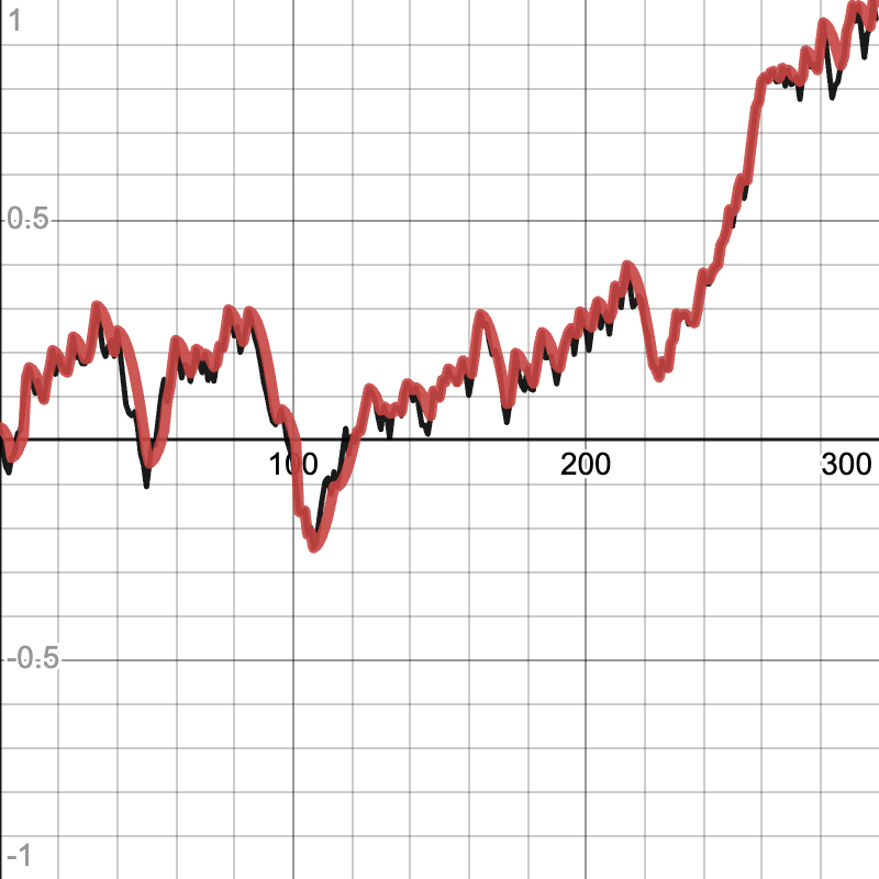
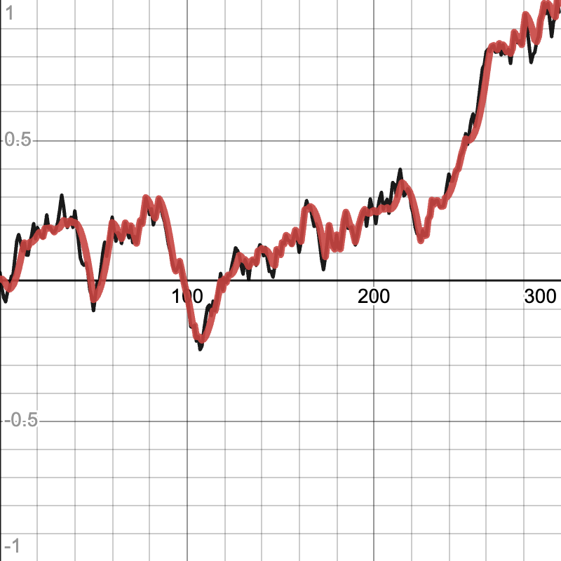
Moving Average

   A simple and effective way of smoothing can be done with a simple moving average (MA).  When given a value in a stream, a MA smoother returns the average of the past n values.  By taking older data into account and averaging it, any noise in that range is reduced because of the average.

   The code given runs in constant time by maintaining an array of the n most recent values and tracking the sum of those values.  The array acts as a queue (more specifically, a circular queue).  When a new value is pushed, it is added to the sum, the oldest value is subtracted from the sum, and the new value takes the oldest value’s place in the array.  This way, the array is accessed exactly twice per push (and very little math needs to be done), making the operation run in constant time.

   The MA smoother is tuned by altering the number of past values to use in the average (the greater the number of values, the greater the smoothing effect).  Note that as the number of values to remember is increased, the smoothed data will begin to lag behind the input data (take longer to switch from increasing to decreasing / decreasing to increasing, be consistently a few steps under increasing / decreasing data, etc.).

Example of MA smoother (input data in black, smoothed data in red):

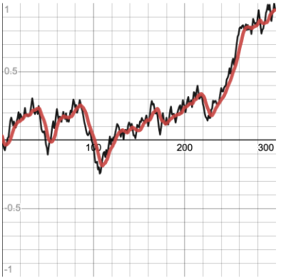
Weighted Moving Average

   A weighted MA is very similar to the MA: the only difference is that a weighted MA can add “weights” to the most recent values.  What these weights do is prioritize the most recent values to adapt to changing data faster.  Mathematically, these weights are multiplied by the most recent values and instead of dividing by the number of values, the sum is divided by the sum of the weights.  For example, if the most recent values are 3, 4, 5, 3, and 4 and the weights are 5 and 3, 5 is multiplied by 3 (the most recent input) and 3 is multiplied by 4 (the next most recent input).  Then the results (15 and 12) are added to the rest of the numbers (which implicitly have a weight of 1 (which is a simple MA)) to make 39.  Then, instead of dividing by 5 (the number of inputs), the sum is divided by 5 plus 3 plus the number of remaining values, 3.  This yields 39 divided by 11 which gived a weighted average of 3.55.

   The code given runs in time proportional to the number of values to remember.  It is possible to write code that runs in time proportional to the number of weights, but I was lazy and time proportional to the number of values to remember is fast enough.  The implementation is very similar to that of the implementation of MA: the weighted MA smoother still maintains an array that acts as a circular queue, but also creates an array of the weights that is padded with ones (which just treats those values as having no weight).  The implementation then adds to the sum the difference between the weight of a value and its next weight times the value.  This is mathematically equivalent to subtracting by the value multiplied by its current weight then adding the value multiplied by its new weight.  This is then done for each value, then the new value is added multiplied by the first weight.  The final weight in the array is 0 so that when the looping is done, the oldest value is subtracted away from the sum completely.  The new value then takes the oldest value’s place in the array of values.

   The Weighted MA smoother is tuned by altering the number of past values to remember and changing the weights.  The first weight in the array is applied to the most recent item, and so on.  Note that as the number of values to remember is increased, the smoothed data will begin to lag behind the input data (take longer to switch from increasing to decreasing / decreasing to increasing, be consistently a few steps under increasing / decreasing data, etc.).  The weighted MA smoother will still smooth as the MA smoother does, but will reflect some finer details in the input data.

Example of weighted MA smoother (input data in black, smoothed data in red):

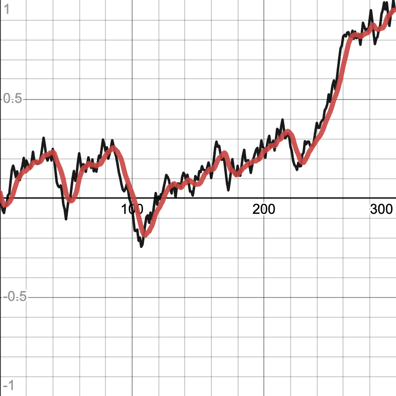
Moving Median

   A moving median (MM) is very similar to MA.  The only difference is that MM is the median (the middle number) of the past n values instead of the average.  As with MA, because past values are taken into account, the data is smoothed.

   The code given runs in time proportional to the number of values to remember.  The implementation uses objects that hold a single double value each.  An array that’s a circular queue of these objects is used to tell which value to forget when the array fills up.  Additionally, a list of the same objects as in the array is maintained to be sorted so the median is trivial to find.  The objects are used so that instead of rebuilding the sorted list with every push and tracking which number in the array corresponds to which value in the list, the internal number of the object automatically changes in the list when it is changed in the array.  Then, sorting the same list (the changed object is still in it) runs quickly because only one object needs to be bubbled to a new position.  When looking at the reset function, it might be noticed that the array is not reset.  This is because the values of the array do not actually matter: only that the objects in it correspond to the objects in the list, and because the list is cleared, those objects hold no meaning afterwards.

   The MM smoother is tuned by adjusting the number of values to remember.  As with the MA smoother, the greater the number of values, the more the smoothed data lags behind the input data.  When comparing the graphs of MM and MA side by side, it can be noticed that they are very similar except that the MM smoother’s data includes finer details (slightly lagged), which makes its graph slightly less “smooth” compared to the MA smoother’s.

Example of MM smoother (input data in black, smoothed data in red):

Proportional

   A proportion (P) is a simple and effective way of smoothing.  All it does is set its new output to the sum of its last output and the difference between the new value and its last output multiplied by some constant.  This is the equivalent of the “P” in a PID controller.  This smooths because the output always approaches the input, smoothing out any sudden changes.

   The code runs in constant time as it is just a simple math formula.  As the output is the only state of the object that changes, it is the only part that needs to be reset.

   The P smoother is tuned by altering the P factor (the percent of the error to change by).  A value of 1 will match the input data exactly, and a value of 0 will keep the output at 0.  The closer the P value to 1, the less smoothing will be done (the output will adapt to the input quicker).

Example of P smoother (input data in black, smoothed data in red):

Fall (Limit Second Derivative)

   The fall smoother will seem very scary in code, but is actually very simple.  All it does is limit the second derivative of the output as it tries to match the input.  Or in other words, the rate of change of the rate of change is limited.  Or in other words, if you draw a line between the previous two points, the line between the previous point and the next one cannot make an angle with the other line that exceeds a predetermined number.  This creates a falling effect when the input data changes too sharply, because the rate of change of the output changes at a constant rate.  The smoother has a fall up parameter that when set to true limits the second derivative when heading away and to zero.  When set to false, the falling will only occur when the input data drops towards zero.

   The code given runs in constant time and tracks the output and the current rate of change.  The first check is whether the output has shot away from zero of the input, which then the tracked rate of change is set to zero to prevent the output from oscillating.  Then the change of the rate of change is computed.  The next check is whether the rate of change of the rate of change (the previously computed value) should be limited.  The right side of the and checks if falling up is allowed or if the input is falling towards zero; the left side of the and checks if the rate of change of the rate of change is greater than the given limit.  If so, then set the rate of change to the rate of change to the limit.  Next, the tracked rate of change is changed by its rate of change (that value), and the output is changed by the new rate of change.  The final check is to again prevent oscillation by checking if the new output is aimed away from zero and if the new output is further away from zero than the input.  If so, the new output is brought back to the input.

   The fall smoother is tuned by changing the maximum second derivative and specifying if falling up should be allowed.  The greater the maximum second derivative, the less smoothing is done.  The lesser the maximum second derivative, the smoother the output is (and longer the “fall”).  Note that this smoother can produce output that matches the input exactly until steep changes if a large enough maximum second derivative is chosen.  If no smoothing is done, the chosen value is too high.

Example of fall smoother with falling up (input data in black, smoothed data in red):

Example of fall smoother without falling up (input data in black, smoothed data in red):